The Laplace and Poisson equations

Introduction

The Laplace equation is given by For example, in Cartesian coordinates and 2D, this becomes The inhomogeneous version of this equation is the Poisson equation, and again, in 2D Cartesian, we have

The Laplace equation

The equation of conservation of mass is also called the continuity equation and it is given by

If density does not change with time, we have

Now we can define a potential function , such that . The conservation of mass is then that is, the Laplace equation. This means that by solving the Laplace equation, we can find the solution for an incompressible inviscid flow.

Solving the Laplace equation with finite differences

Code used for this lecture

(warning: it is listed as 'poisson_*.f90' but it actually solves the Laplace equation)

The method of finite differences essentially consists of "inflating" infinitesimal differentials into differences. For example, consider the definition of the first derivative of a function

A finite difference approximation of this derivative would therefore be , where .

Now let's return to our problem of the Laplace equation, and use as meaning the same as . Those are abuses of notation which only intend to make coding easier.

Using finite differences,

we set . Then, using indices,

This can be represented in stencil notation in the computational grid as

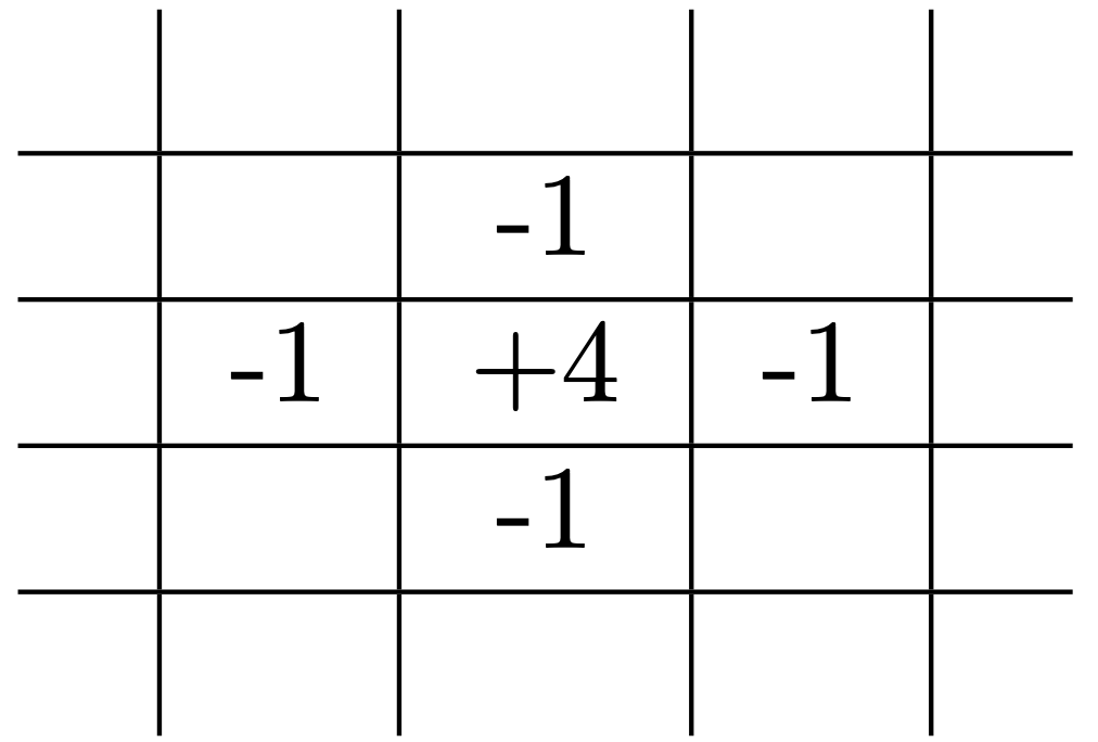
As an example, for a grid we have for the cell at the center

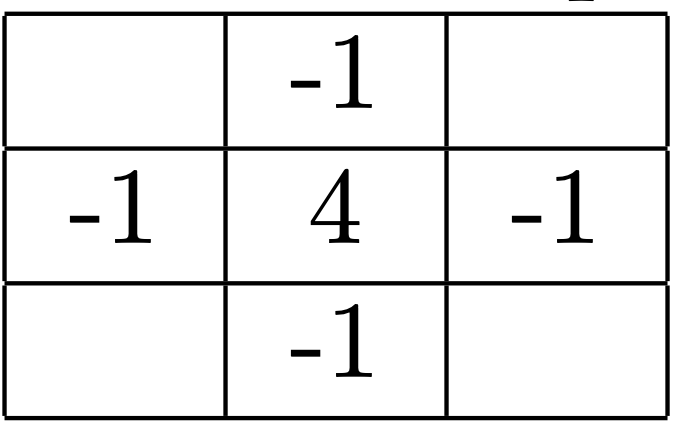
If we deconstruct this grid, putting rows one after another, we can write the Poisson equation applied at the cell at the center

So, we get a ``dot product'' notation.

The cells of the grid represent only the inner points of the whole computational domain. That is why we enumerated them as . The cells with indices 0 and 4 are the boundaries. In order to use the same ``dot product'' notation as above, we can just put the boundary values at the right hand side of the equation. So, for , we would have

So, this means that we can continue with the same pattern that we used for the cell at the center, and we put the boundary cells in the right-hand side. When we have all equations for all cells, we can solve the system of equations for all the unknowns. We can write the system in matrix notation.

Matrix notation for the solution

Now, we stack all the equations together in a matrix. For our grid,

The matrix (that we will call ) is a block matrix of the following form (we show an example for a grid)

where is the identiy matrix and

The equation is in the form The vector contains the unknowns of the system, and vector contains the known boundary conditions.

For a given cell , we shall think of the row that has the positive value () as the coefficient of as the row that is supposed to calculate the value of , and we can think of the negative coefficients as the values of the neighbouring cells that are necessary to determine the value of .

The continuation of this problem is in the documentation of the Github repository. Although this is the basis for solving the Laplace equation, and effective implementation needs to do the following additional steps, which are more technical in nature:

• Create an indexing system for all the cells in the computational domain
• Define the boundary conditions for a given problem.

We will apply this implementation to solve two problems:

• A uniform, free flow
• An obstacle in a fluid flow

The uniform free flow

In the case of a uniform free flow, it is useful to discuss here the analytical solution in order to compare later.

If the fluid flows from left to right,

this means from the definition of ,

We get linear flow lines, which follow the gradient of f. In particular, if we set the integration constant to zero, we see what happens at the boundaries:

• At the left boundary, where , then .
• At the right boundary, where , then , i.e., a constant.
• At the top and bottom boundaries, we get a variable value of f, i.e., .

The Poisson equation

Self-gravity can be expressed as

This can be introduced into an astrophysics problem in several situations:

• As a 1D spherical problem
• As a particle force problem (N body computations, for example for orbits)
• As a 2D or 3D problem in either Cartesian, cylindrical or spherical coordinates.

A 1D spherical problem

The easiest procedure in this case is to directly compute the gravitational force with the enclosed mass, that is . That is,

where is the enclosed mass. In the case of a spherically symmetric mass distribution in spherical coordinates, .

Particle methods

In an N-body problem, the gravitational force between two particles of masses and is

The total force on a particle can be computed by summing over all other particles, i.e., .

If the particles are very close to each other, then the denominator can become very small and the forces increase a lot. Then the accelerations increase and the time steps in the simulation increase (the simulation freezes). Imagine we are modeling a system where close encounters are considered rare (for example, stars in the collision of two galaxies). Then, we can introduce a softening parameter :

The softening parameter is arbitrary and it adds to the free degrees of a system (which is not necessarily what one wants when researching the solution of a problem).

2D or 3D problem

In Cartesian coordinates, the Poisson equation becomes

if we only consider , we have

using finite differences like in the Laplace equation, and letting , we have

Again, this equation can be written as a matrix equation with given boundary conditions, for example

• Periodic boundaries: useful when simulating part of a bigger structure, for example, for cosmological simulations;
• Zero: technically, zero is not a good value for the boundary since only for the gravitational potential should go to zero under usual normalizations;
• Monopole: if matter is mostly contained in a central region of the simulation box, then , where is the total mass;
• Multipole: if the mass distribution cannot be approximated as a point mass but the distribution can be expanded in terms of multipoles for , this expansion can be used as a boundary condition.

The problem is how to invert this matrix. In our simple example for the Laplace equation, we make the inversion directly. However, this is very costly, and faster methods are available, for example:

• Use of Fourier transforms
• Polynomial expansions

Study case: self-gravity module for PLUTO. Method paper