Given a second-order differential operator , a function and , the differential equation
subject to boundary conditions, defines an eigenvalue problem (a problem such that a scalar has the same effect on as an operator ). Compared to linear algebra of matrices, the differential operator is equivalent to a matrix and the functions are equivalent to eigenvectors (here called eigenfunctions). The functions subject to the boundary conditions form a Hilbert space. The operator has a general form
where we limit ourselves to the case , .
Example: The spatial part of a standing wave must satisfy the differential equation subject to the boundary conditions . Defining , one has . The eigenvalues are then . The solutions to this equation are the eigenfunctions , with , . We can show that these functions are orthogonal, i.e., within the interval .
Hermitian adjoint operator
Consider the inner product of two functions, , where is a differential operator acting on . An adjoint operator is defined such that plus extra terms due to the boundaries. If those extra terms are zero, then the operator is called Hermitian adjoint. (Remember that the inner product has the complex conjugate defined, as well as an interval and a weight!)
Self-adjoint operator
An operator for which . A Hermitian self-adjoint operator is simply called Hermitian. It can be shown that is self-adjoint if . This means that one can write .
Hermitian adjoint operator
Consider the inner product of two functions, , where is a differential operator acting on g. An adjoint operator is defined such that + extra terms due to the boundaries. If those extra terms are zero, then the operator is called Hermitian adjoint. (Remember that the inner product has the complex conjugate defined, as well as an interval and a weight!)
Self-adjoint operator
An operator for which . A Hermitian self-adjoint operator is simply called Hermitian. It can be shown that is self-adjoint if . This means that one can write .
Orthogonality of the eigenfunctions
Case without weight function
Consider a Hermitian operator that satisfies , , where and no weight. Then,
= (int. by parts)
= (another int. by parts) =.
The boundary terms must vanish if is Hermitian, by definition. We see that if are eigenfunctions, we can write
For and in general , and if the boundary terms vanish, then (i.e, the eigenfunctions must be orthogonal).
Case with the weight function
If the operator is not self-adjoint ("nsa"), then there can be a function (the weight function) such that, when , it makes the operator self-adjoint (sa) (i.e., ). One can show that such a function is . The equation becomes
and after the same procedure as the case without the weight function, we find meaning that the inner product requires the weight function for the functions to be considered orthogonal.
Building the Sturm-Liouville problem
The second-order linear ordinary differential equation
with the Hermitian operator , subject to suitable boundary conditions, is called a Sturm-Liouville problem. (Note: from now on, )
The boundary conditions must be such that for two eigenfunctions. There are several possibilities. For real eigenfunctions, here are some examples:
Dirichlet boundary conditions:
Neumann boundary conditions:
Periodic boundary conditions:
Other combinations of the eigenfunctions or their derivatives such that the term in the parenthesis is zero at the boundaries
Making to be zero at the boundaries.
Series expansion of a function
One can develop a given function into a series (i.e., set the function as the limit value to which the series must converge) of a set of (orthogonal) eigenfunctions () that form the basis of a vector space:
The limit of the series can be, e.g., from to , or from to . If the eigenfunctions are not orthonormal, one can find the normalization constant as . The coefficients can be found using the inner product (multiplying from the right by with a different index ):
( is the Kronecker delta).
Classical orthogonal polynomials
There are some orthogonal polynomials that satisfy the Sturm-Liouville equation and are called classical orthogonal polynomials. Remember: there are functions that satisfy the Sturm-Liouville equation and that are not polynomials.
Generalized Rodrigues's formula
Where:
is a polynomial of degree with only real roots
strictly positive function ("weight function"), integrable within and such that
is a first-degree polynomial in .
The generalized Rodrigues's formula generates classical orthogonal polynomials in the interval . The constant depends on the standard normalization of the polynomials (chosen so for historical reasons).
Note: It can be proven that the Rodrigues's formula generates polynomials that satisfy the differential equation , i.e., they satisfy a Sturm-Liouville problem.
Generating function: it is also possible to generate all orthogonal polynomials that satisfy a given Sturm-Liouville problem by repeated differentiations of a generating function that can be expanded as with some constants . Note that the nth derivative w.r.t. brings out the polynomials and changes of variables to the index in the series create terms like or . This means that derivatives of the generating function can create recurrence relations.
Schläfli representation
In order to extend the definition of orthogonal polynomials to the complex plane, we start by the complex Rodrigues's formula, ,
where , ( because is a polynomial).
Using Cauchy's integral formula
to integrate times, we find
where encloses the point , and the numerator inside the integral is analytic on and within .
The following examples require the knowledge of: Legendre polynomials, elliptic integrals and Bessel functions.
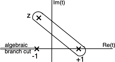
Example: contrary to the Rodrigues's formula, the Schläfli representation doesn't need to make sense. Therefore, one can use the Schläfli representation for generalizing a polynomial to a function with non-integer values of . As a concrete example, consider the Legendre polynomials. Substituting from the table, we find . The contour is in the figure. Generalizing for and using the change of variable , it is possible to show that can be written as an elliptical integral , which is another kind of special function. Integral representations are useful for finding relations (sometimes unexpected) between special functions.
Example: Schläfli integral for non-polynomials and its relation to generating functions. The Bessel functions of the first kind are not polynomials, but they have a generating function (see table). If we apply the residue theorem to an integral containing the generating function, we get with C encircling . With the change of variable , and being the unit circle, we find in general for or for . In this case, the generating function was used to get (a) Schläfli representation, but we can also derive generating functions (for example, for polynomials) using the/a Schläfli representation.
References
Dennery, P., Krzywicki, A. (1967) Mathematics for Physicists. Dover publications.
Lang, C.B., Pucker, N. (2016) Mathematische Methoden in der Physik (3.ª ed., en alemán). Springer.
Hassani, S. (1999) Mathematical Physics. Springer.
Korn, G.A.; Korn, T.M. (1968) Mathematical handbook for scientists and engineers. Dover publications.
Boas, M. (1983) Mathematical Methods in the Physical Sciences. Wiley.